On the optimal water flow velocity in heating network pipelines

Current recommendations regarding the optimal water flow velocity in district heating pipelines (up to 3 m/s) and permissible specific pressure drops R (up to 80 Pa/m) [1] are primarily based on techno-economic calculations. These calculations account for the fact that increasing the flow velocity reduces pipeline cross-sections and the required volume of thermal insulation—thereby lowering capital expenditures for network construction—while simultaneously increasing operational costs for water pumping due to higher hydraulic resistance (and vice versa). Consequently, the optimal velocity corresponds to the minimum total discounted cost over the system’s design depreciation period.

However, in a market economy, it is essential to account for the discounting of both operational costs E (RUB/year) and capital expenditures K (RUB). In this context, the formula for calculating total discounted costs (TDC)—when borrowed funds are utilized—is expressed as follows [2]:

In this case – discount factors for capital and operating costs, calculated based on the estimated amortization period $T$ (in years) and the discount rate $p$. The latter accounts for the inflation rate and investment risks—reflecting, ultimately, the degree of economic instability and the nature of fluctuations in current tariffs—and is typically determined using expert estimation methods [2]. As a first approximation, the value of $p$ corresponds to the annual interest rate on a bank loan. In practice, it can be taken as the refinancing rate set by the Central Bank of the Russian Federation; as of January 15, 2004, this rate is 14% per annum.

It is not known a priori whether the minimum total discounted cost will correspond to the same water velocity and specific loss levels recommended in the literature [1]. Therefore, it is advisable to perform new calculations using current price ranges for pipelines, thermal insulation, and electricity. Assuming that the pipelines operate under a quadratic resistance regime and calculating specific pressure losses using the formulas provided in the literature [3], the optimal water velocity can be determined by the following formula:

Here, К_ти is the cost-increase factor for pipelines due to the presence of thermal insulation. When using domestic materials such as mineral wool mats, К_ти = 1.3 can be taken. The C_D parameter represents the specific cost of one meter of pipeline (rubles/m2), related to the internal diameter D_м. Since price lists typically specify the cost of metal C_м in rubles per ton, the conversion must be performed using the following straightforward relationship:, where– pipeline wall thickness (mm), =7,8 т/м³ – density of the pipeline material. Value С_эл corresponds to the electricity tariff. According to data from OAO Mosenergo for the first half of 2004, for residential/utility consumers С_эл= 1,1723 руб./кВтч.

Formula (2) is derived from the condition d(TCO)/dv = 0. In determining operational costs, it was assumed that the equivalent pipe-wall roughness is 0.5 mm [3] and that the efficiency of the network pumps is approximately 0.8. The density of water, ρw, was taken as 920 kg/m³ for the typical temperature range found in a heating network. Furthermore, it was assumed that circulation within the network is maintained year-round—an assumption that is well-justified given the requirements for hot water supply.

An analysis of formula (1) shows that for long depreciation periods T (10 years or more), which are typical for heating networks, the ratio of the discount factors is practically equal to its lower limiting value, p/100. In this case, expression (2) yields the lowest economically justifiable water velocity—a value corresponding to the condition where the annual interest on a construction loan equals the annual savings in operating costs (i.e., an infinite payback period). For a finite payback period, the optimal velocity would be higher. In any event, however, this velocity will exceed the value calculated without accounting for discounting, since, as can be easily shown, , and under current conditions, it turns out that 1/T < p/100.

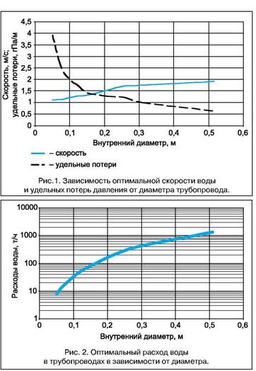
Values for optimal water velocity and the corresponding appropriate specific pressure losses, calculated using expression (2) at an average C_D level and a limiting ratio,…are shown in Fig. 1. It should be noted that formula (2) includes the parameter D, which is not known in advance; therefore, it is advisable to first assume an average velocity (on the order of 1.5 m/s), determine the diameter based on the specified water flow rate G (kg/h), and then calculate the actual velocity. and the optimal speed according to (2) and check whether v_ф will be greater than vопт. If not, the diameter should be reduced and the calculation repeated. It is also possible to obtain the relationship directly between G and D. For the average C_D level it is shown in Fig. For an average C_D value, this is shown in Fig. 2.

Thus, the economically optimal water velocity in heating networks, calculated for the conditions of a modern market economy, does not, in principle, fall outside the ranges recommended in the literature [1]. However, this velocity is less dependent on pipe diameter than it would be if based on criteria for permissible specific pressure losses; for small and medium diameters, higher values of R-up to 300–400 Pa/m—prove to be advantageous. Consequently, it is preferable to further reduce capital expenditures (in this context, by decreasing pipe cross-sections and increasing water velocity)—a preference that becomes more pronounced as the discount rate rises. Therefore, the tendency—often observed in practice—to minimize initial investment costs when installing engineering systems finds a theoretical justification.

Literature

1. A. A. Ionin et al. Heat Supply. Textbook for Higher Education Institutions. — Moscow: Stroyizdat, 1982, 336 p.

2. V.G. Gagarin. Criterion for the Payback of Costs for Improving the Thermal Protection of Building Envelopes in Various Countries. In: Proceedings of the NIISF Conference, 2001, pp. 43–63.

3. SNiP 2.04.07-86* “Heating Networks”. – Moscow: GUP TsPP, 1998.

Based on material from the journal *Novosti Teplosnabzheniya* (Heat Supply News), No. 1, 2005, www.ntsn.ru
Copyright held by:
O. D. Samarin, Candidate of Technical Sciences, Associate Professor,
Moscow State University of Civil Engineering